Flow Matching - A Generalized Framework for Diffusion Model?

Continuous Normalizing Flows (CNFs), a special kind of generative model has gained attention for its ability to transform simple data patterns into complex ones seamlessly. In this blog post, we will explore the workings of CNFs, understand the innovations brought by its variations and its deep connection with diffusion models. The goal is to showcase how these methods are pushing the boundaries of generative modeling, making it more stable, efficient, and versatile.

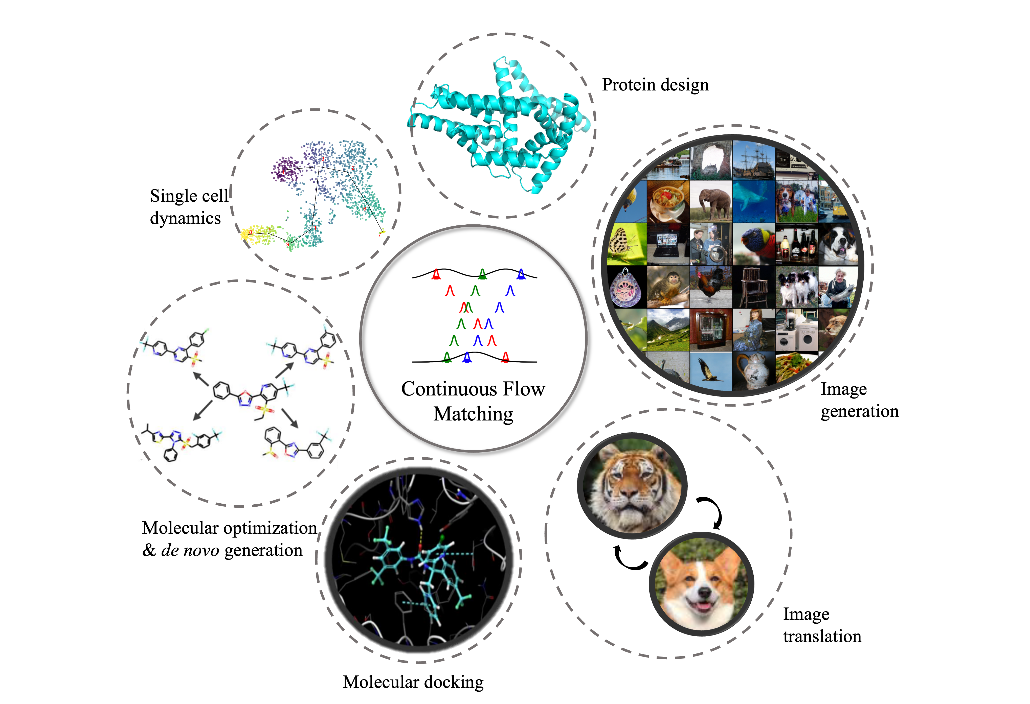
Continuous Normalizing Flows (CNFs)

In the realm of Continuous Normalizing Flows (CNFs), we operate in a $d$-dimensional data space, denoted as $\mathbb{R}^d$, with data points represented as $x=\left(x^1, \ldots, x^d\right)$. Two crucial elements in this context are:

Probability Density Path, $p[0,1] \times \mathbb{R}^d \rightarrow \mathbb{R}_{>0}$: A function that gives us a timedependent probability density for each point in our data space. Fol any given time $t$, the integral of $p_t(x)$ over the entire data space equals 1.
Vector Field, $v:[0,1] \times \mathbb{R}^d \rightarrow \mathbb{R}^d$ : A time-dependent function that points us in the direction we need to move in our data space: $v_t(x)=\frac{d x}{d t}$.

Their relationship can be categorized by the continuity equation:

\[\frac{\partial p_t}{\partial t}=-\nabla \cdot\left(p_t u_t\right)\]

The Flow and Its Transformation

A Continous Normalizing Flow (CNF) is a special kind of flow where the vector field $v_t$ is modeled by a neural network with parameters $\theta$. This results in a deep, learnable model of our transformation $\phi_t$, allowing us to reshape a simple initial density $p_0$ (like pure noise) into a more complex one, $p_1$, through the push-forward equation:

\[p_t=\left[\phi_t\right]_* p_0\]

Here, the push-forward operator $*$ is defined as:

\[\left[\phi_t\right]_* p_0(x)=p_0\left(\phi_t^{-1}(x)\right) \cdot \operatorname{det}\left[\frac{\partial \phi_t^{-1}}{\partial x}(x)\right]\]

This equation essentially tells us how the probability density at any point in our data space changes as we follow the flow.

Generating Probability Density Paths

A vector field $v_t$ is said to generate a probability density path $p_t$ if its flow $\phi_t$ satisfies the push-forward equation. In practice, we can use the continuity equation to check if a given vector field generates a probability path, which is a crucial aspect of the theoretical foundation of CNFs.

💡TIP

The flow $\phi$ and the vector field $v$ are bidirectional, i.e.

Flow $\phi$ determines the vector field $v$

Vector field $v$ determines the flow $\phi$

The probability density path $p$ can also be determined by flow/vector field. However, the inverse is not staightforward. In most cases, there might be different flows/vector fields that lead to the same probability density path. There are many recent works on continous flow matching exploring different possible flows/couplings under the same probability density path for better training and inference effiency

Dive into Conditional Flow Matching (CFM)

In the realm of generative modeling, we often deal with an unknown data distribution $q\left(x_1\right)$ from which we can sample, but whose density function is inaccessible. Our goal is to transform a simple distribution $p_0$ (e.g., a standard normal distribution $\mathcal{N}(x \mid 0, I)$) into a distribution $p_1$ that closely approximates $q$. This transformation is represented by a probability path $p_t$, where $t$ ranges from 0 to 1.

Flow Matching Objective

The Flow Matching (FM) objective is designed to facilitate this transformation, guiding the flow from $p_0$ to $p_1$. Mathematically, it is defined as:

\[\mathcal{L}_{\mathrm{FM}}(\theta)=\mathbb{E}_{t, p_t(x)}\left\|v_\theta(t, x)-u_t(x)\right\|^2\]

Here, $\theta$ represents the learnable parameters of the CNF vector field $v_t$ , and $u_t(x)$ is a target vector field that generates the probability path $p_t(x)$. The expectation is taken over a uniform distribution of $t$ and the distribution $p_t(x)$.

Challenges and Tractability

While the FM objective is conceptually straightforward, it poses practical challenges. The main issue is that we don’t have prior knowledge of an appropriate $p_t$ and $u_t$, making the direct application of FM intractable.

Conditional Flow Matching Objective

To address this, Lipman et al, 2023 first introduce conditional probability paths $p_t\left(x \mid x_1\right)$ and corresponding vector fields $u_t\left(x \mid x_1\right)$. These are defined per data sample $x_1$, and by aggregating them, we can construct the desired $p_t$ and $u_t$. The aggregation is done through marginalization:

\[\begin{gathered} p_t(x)=\int p_t\left(x \mid x_1\right) q\left(x_1\right) d x_1 \\ u_t(x)=\int u_t\left(x \mid x_1\right) \frac{p_t\left(x \mid x_1\right) q\left(x_1\right)}{p_t(x)} d x_1 \end{gathered}\]

A more tractable objcetive, called Conditional Flow Matching (CFM) is then introduced as:

\[\mathcal{L}_{\mathrm{CFM}}(\theta)=\mathbb{E}_{t, q\left(x_1\right), p_t\left(x \mid x_1\right)}\left\|v_\theta(t,x)-u_t\left(x \mid x_1\right)\right\|^2\]

CFM allows for unbiased sampling and efficient computation, as it operates on a per-sample basis. This appraoch is grounded in two key observations:

Marginal Vector Field Generates Marginal Probability Path: The aggregated vector field $u_t(x)$ correctly generates the marginal probability path $p_t(x)$, establishing a connection between conditional and marginal vector fields.
Equivalence of Gradients: The gradients of the FM and CFM objectives with respect to $\theta$ are identical, meaning that optimizing CFM is equivalent to optimizing FM.

Click here to know details

Statement: If $p_t(x)>0$ for all $x \in \mathbb{R}^d$ and $t \in[0,1]$, then up to a constant independent of $\theta, \mathcal{L}_{\mathrm{CFM}}$ and $\mathcal{L}_{\mathrm{FM}}$ are equal, implying that

\[\nabla_\theta \mathcal{L}_{\mathrm{FM}}(\theta)=\nabla_\theta \mathcal{L}_{\mathrm{CFM}}(\theta)\]

Proof: Begin by stating the assumptions and preliminaries: We assume that $q$, $p_t(x \mid z)$ decrease to zero sufficiently quickly as $\|x\| \rightarrow \infty$, and that $u_t$, $v_t$, $\nabla_\theta v_t$ are bounded.

Starting with the gradients of the expected values involved in $\mathcal{L}_{\mathrm{FM}}$ and $\mathcal{L}_{\mathrm{CFM}}$, we have the following equalities:

\[\begin{aligned} \nabla_\theta \mathbb{E}_{p_t(x)}\left\|v_\theta(t, x)-u_t(x)\right\|^2 & =\nabla_\theta \mathbb{E}_{p_t(x)}\left(\left\|v_\theta(t, x)\right\|^2-2\left\langle v_\theta(t, x), u_t(x)\right\rangle+\left\|u_t(x)\right\|^2\right) \\ & =\nabla_\theta \mathbb{E}_{p_t(x)}\left(\left\|v_\theta(t, x)\right\|^2-2\left\langle v_\theta(t, x), u_t(x)\right\rangle\right) \\ \end{aligned}\] \[\begin{aligned} \nabla_\theta \mathbb{E}_{q(z), p_t(x \mid z)}\left\|v_\theta(t, x)-u_t(x \mid z)\right\|^2 & =\mathbb{E}_{q(z), p_t(x \mid z)} \nabla_\theta\left(\left\|v_\theta(t, x)\right\|^2-2\left\langle v_\theta(t, x), u_t(x \mid z)\right\rangle+\left\|u_t(x \mid z)\right\|^2\right) \\ & =\mathbb{E}_{q(z), p_t(x \mid z)} \nabla_\theta\left(\left\|v_\theta(t, x)\right\|^2-2\left\langle v_\theta(t, x), u_t(x \mid z)\right\rangle\right) . \end{aligned}\]

Here, we used the bilinearity of the dot product and the fact that $u_t$ does not depend on $\theta$.

Next, we show that the expected values of certain functions under $p_t(x)$ and $q(x_1)p_t(x \mid x_1)$ are equal:

\[\begin{aligned} \mathbb{E}_{p_t(x)}\left\|v_\theta(t, x)\right\|^2 & =\int\left\|v_\theta(t, x)\right\|^2 p_t(x) d x \\ & =\iint\left\|v_\theta(t, x)\right\|^2 p_t(x \mid x_1) q(x_1) d x_1 d x \\ & =\mathbb{E}_{q(x_1), p_t(x \mid x_1)}\left\|v_\theta(t, x)\right\|^2 \end{aligned}\] \[\begin{aligned} \mathbb{E}_{p_t(x)}\left\langle v_\theta(t, x), u_t(x)\right\rangle & =\int\left\langle v_\theta(t, x), \frac{\int u_t(x \mid x_1) p_t(x \mid x_1) q(x_1) d x_1}{p_t(x)}\right\rangle p_t(x) d x \\ & =\iint\left\langle v_\theta(t, x), u_t(x \mid x_1)\right\rangle p_t(x \mid x_1) q(x_1) d x_1 d x \\ & =\mathbb{E}_{q(x_1), p_t(x \mid x_1)}\left\langle v_\theta(t, x), u_t(x \mid x_1)\right\rangle . \end{aligned}\]

For the first equality, we utilized the law of total expectation, and for the second, we applied Bayes’ theorem followed by a change of the order of integration.

Putting it all together, since the gradients of $\mathcal{L}_{\mathrm{FM}}$ and $\mathcal{L}_{\mathrm{CFM}}$ are the same at all times $t$, it follows that $\nabla_\theta \mathcal{L}_{\mathrm{FM}}(\theta) = \nabla_\theta \mathcal{L}_{\mathrm{CFM}}(\theta)$, up to a constant independent of $\theta$. This completes the proof.

A Simple Case: Vanilla CNF

Let’s consider the most simple case in generative modeling, where we need to transform a normal distrbution to the data distribution. As previously established, FM objectives and be replaced with tractable CFM objectives. Consequently, our next step is to construct a conditional flow denoted as $\psi_t\left(x \mid x_1\right)$. This flow needs to be meticulously designed to satisfy two boundary conditions: the corresponding marginal distribution should approximate the data distribution when $t\rightarrow 1$, and revert to approximating a normal distribution when $t\rightarrow 0$

Lipman et al, 2023 propose a very simple form of flow which is conditioned on $x_1$ and can satisfy the above requirements:

\[\psi_t(x)={\color{plum}\sigma_t\left(x_1\right)} x+{\color{plum}{\mu_t}\left(x_1\right)}\]

Under this formulation, the evolving conditional probability path is represented by a Gaussian distribution, characterized by a time-dependent mean $\mu_t(x_1)$ and time-dependent variance $\sigma_t(x_1)$:

\[p_t\left(x \mid x_1\right)=\mathcal{N}\left(x \mid \mu_t\left(x_1\right), \sigma_t\left(x_1\right)^2 I\right)\]

Specifically, if we let $\mu_{t \rightarrow 1}\left(x\right) \rightarrow x, \mu_{t \rightarrow 0}\left(x\right) \rightarrow 0$ and $\sigma_{t\rightarrow 0}\left(x\right) \rightarrow 1, \sigma_{t\rightarrow 1}\left(x\right) \rightarrow \sigma_\text{min}$, then it will approximate normal distribution ($t \rightarrow 0$) and data distribution ($t \rightarrow 1$). Here the term $\sigma_\text{min}$ is considered to be sufficiently small to mimic characteristics of the Dirichlet distribution, further aligning the model with the data distribution’s behavior.

In Lipman et al, 2023, they directly choose the linear interpolation, which result in

\[\mu_t(x)=t x_1, \text { and } \sigma_t(x)=1-\left(1-\sigma_{\min }\right) t\]

With continuity equation, we can finally get the conditional vector field and the training objectives:

\[\begin{align*} u_t\left(x \mid x_1\right)&={\color{skyblue}\frac{\sigma_t^{\prime}\left(x_1\right)}{\sigma_t\left(x_1\right)}\left(x-\mu_t\left(x_1\right)\right)+\mu_t^{\prime}\left(x_1\right)} && {\color{skyblue}\text{(definition)}}\\ &=\frac{x_1-\left(1-\sigma_{\min }\right) x}{1-\left(1-\sigma_{\min }\right) t} && \text{(substituting)}\\ \mathcal{L}_{\mathrm{CFM}}(\theta)&= \mathbb{E}_{t, q\left(x_1\right), p\left(x \mid x_1\right)}\left\|v_\theta\left(x_1, t\right)-u_t\left(x \mid x_1\right)\right\|^2\\ &=\mathbb{E}_{t, q\left(x_1\right), p\left(x \mid x_1\right)}\left\|v_\theta\left(x_1, t\right)-\frac{x_1-\left(1-\sigma_{\min }\right) x}{1-\left(1-\sigma_{\min }\right) t}\right\|^2 \end{align*}\]

For sampling, we first draw a random noise from normal distribution $x_0 \sim \mathcal{N}(0, I)$ and then reversely solve the differential equation $d x=v_\theta(t, x) d t$, where $v_\theta(t, x)$ is learned force field.

Relation to Diffusion Models

💡TIP

(For consistency with flow matching concepts, we exchange the timestep notation by previous literature, i.e. the forward diffusion process is $p_1 \rightarrow p_0$ and the denoising process is $p_0 \rightarrow p_1$)

Reflecting on diffusion models, they incrementally introduce noise into the data. This process of adding noise can be interpreted as an interpolation between the data and the noise distribution, which aligns with the concept of flow in continuous flow matching.

Fig 1 from Lipman et al, 2023: Comparison of the conditional interpolation paths in vanilla flow matching (left) and vanilla diffusion (right).

Moreover, the training objective of a diffusion model is to approximate the conditional score function $\nabla\log p_t (x\mid x_1)$, where the score function can be reparameterized as the prediction of the denoised data $x_1$ (denoised data). This is parallel to flow matching, where the prediction (or vector field) can likewise be reparameterized as the prediction of $x_1$:

\[\begin{aligned} \nabla \log p_t\left(x \mid x_1\right) =\frac{x-\alpha_{1-t} x_1}{1-\alpha_{1-t}^2} \overset{\text{reparam.}}{\longleftrightarrow} & x_1 && \text{(VP Diffusion)}\\ u_t\left(x \mid x_1 \right) =\frac{x_1-\left(1-\sigma_{\min }\right) x}{1-\left(1-\sigma_{\min }\right) t} \overset{\text{reparam.}}{\longleftrightarrow} & x_1 && \text{(Vanilla CNF)} \end{aligned}\]

Consequently, diffusion models can be seen as specific cases of continuous flow matching. Below are two examples illustrating how flow matching is constructed from diffusion models:

Example: Variance Preserving Diffusion

In variance preserving (VP) diffusion, the conditional noisy distribution in the forward process is given by:

\[p_t\left(x \mid x_1\right)=\mathcal{N}\left(x \mid \alpha_{1-t} x_1,\left(1-\alpha_{1-t}^2\right) I\right), \text { where } \alpha_t=e^{-\frac{1}{2} T(t)}, T(t)=\int_0^t \beta(s) d s\]

To align this with the conditional probability path in CNF, the corresponding conditional flow and vector field are:

\[\begin{align*} \psi_t(x)&=\sqrt{1-\alpha_{1-t}^2} x+\alpha_{1-t} x_1\\ u_t\left(x \mid x_1\right)&=\frac{\alpha_{1-t}^{\prime}}{1-\alpha_{1-t}^2}\left(\alpha_{1-t} x-x_1\right) \end{align*}\]

Example: Variance Exploding Diffusion

In variance exploding (VE) diffusion, the conditional noisy distribution in the forward process is:

\[p_t\left(x \mid x_1\right)=\mathcal{N}\left(x \mid x_1, \sigma_{1-t}^2 I\right), \text{ where } \sigma_0 \ll 1, \text { and } \sigma_1 \gg 1\]

Again, aligning this with the conditional probability path in CNF, the corresponding conditional flow and vector field are:

\[\begin{align*} \psi_t(x)&=\sigma_{1-t} x+ x_1\\ u_t\left(x \mid x_1\right)&=-\frac{\sigma_{1-t}^{\prime}}{\sigma_{1-t}}\left(x-x_1\right) \end{align*}\]

Bridging Diffusion and Flow with the Probability Flow ODE

Another perspective on their similarity is via the Probability Flow ODE introduced in Lipman et al, 2023. Consider the SDE framework in diffusion models:

\[d x=f_t d t+g_t d w\]

where $f_t$ is the drift term and $g_t$ is the diffusion term. The time-dependent probability density $p_t(x)$ is governed by the Fokker-Planck equation:

\[\begin{align*} \frac{d p_t}{d t} & = -\operatorname{div}\left(f_t p_t\right)+\frac{g_t^2}{2} \Delta p_t && \text{(Fokker-Planck equation)}\\ & =-\operatorname{div}\left(f_t p_t-\frac{g^2}{2} \frac{\nabla p_t}{p_t} p_t\right) && \text{(definition of Laplace operator)}\\ & =-\operatorname{div}\left(\left(f_t-\frac{g_t^2}{2} \nabla \log p_t\right) p_t\right)\\ & =-\operatorname{div}\left(u_t p_t\right) \end{align*}\]

where $u_t=f_t-\frac{1}{2} g_t^2 \nabla \log p_t$ is the vector field that generates the probability density path. By substituting $f_t$ and $g_t$ with parameters from VP/VE diffusion, we derive the same vector field as in the flow matching examples (previous seection). This demonstrates that diffusion models are indeed special cases of continuous flow matching with specific path, where fitting the conditional score function $\nabla \log p_t\left(x \mid x_1\right)$ corresponds to fitting the conditional vector field $u_t$, and inference through flow corresponds to inference through ODE.

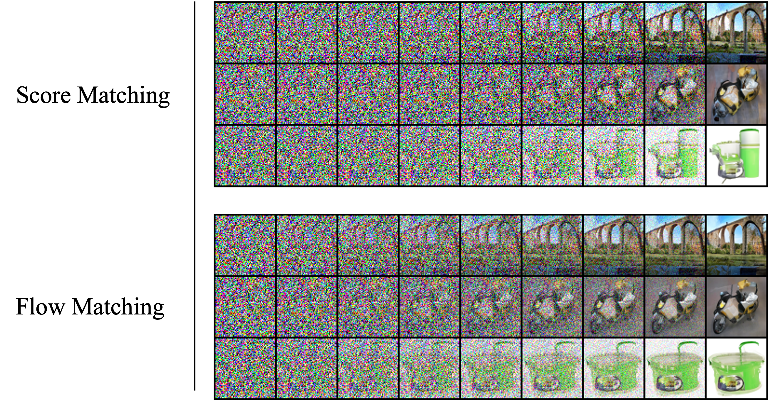
Why Flow Matching Better?

It’s hard to directly explain why flow matching is better than diffusion models from a theoretical perspective. However, we can still find some clues from the following aspects:

Explicit Control Over Probability Paths: The vanilla FM allows for direct control over the entire probability path via the specification of $\mu_t$ and $\sigma_t$. This contrasts with diffusion models (e.g. VE-SDE) where the paths are derived as solutions to diffusion processes and don’t reach a true noise distribution in finite time.
Stability and Robustness in Training: Figure has shown the training objectives (score function/vector field) in a simplified gaussian case. It’s observed that compared with diffusion, vector field in vanilla CNF (denoted by OT path because of its connection to optimial transport map) has a constant direction, which is more stable and robust in training. This is also confirmed by the experiments in Lipman et al, 2023.

Fig 2 from Lipman et al, 2023: Comparison of diffusion and flow matching objectives in a simplified gaussian case. The score function in diffusion trajectory (left) is unstable and sensitive to noise, while the vector field in vanilla flow matching trajectory (right) is stable and robust.

Efficient Inference: Inference in diffusion models is done by sampling from the noise distribution and then running the reverse SDE. In contrast, inference in flow matching is done by solving the ODE, which is much more efficient. The learning objective of flow matching also directly corresponds to the vector field in the inference process, which is not the case for diffusion models.

Fig 3 from Lipman et al, 2023: Comparison of diffusion and flow matching inference results in image generation.

Flow Matching in Biological Application

The integration of generative models into biological research has brought about innovative methodologies that are transforming the field. The recent surge in the application of flow matching within biological modeling marks a significant advancement. Here we examine seminal works that epitomize this progress:

Protein Design

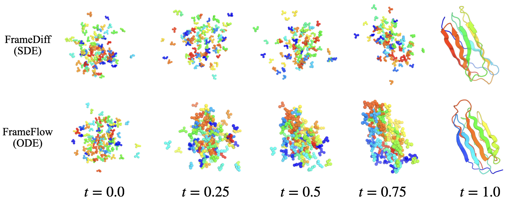
Protein design is a critical problem in computational biology, where the critical step is to generate a proten backbone structure. Yim et al, 2023 proposes a flow-matching generative modeling framework to address this task. The flow matching model is mainly adapted from an existing diffusion model, FrameDiff, where the vector field/score function is defined on SE(3), the group of 3D rotations and translations of residue frame. The learned vector field can then be used to generate protein backbone structures by solving the ODE. Briefly, their framework can be summarized as:

Extanding Flowing Matching on SE(3): In their work, they follow the residue representation introduced by AlphaFold2, where residue are represented by 3D rotations and translations, i.e. $\mathbf{T} \in \operatorname{SE}(3)^N$. Each frame $T=(r, x)$ consists of a rotation $r \in \mathrm{SO}(3)$ and a translation vector $x \in \mathbb{R}^3$. The flow is then defined as geodesic paths connecting the initial and final configurations in SE(3):

\[\begin{align*} &\text{Translations} \left(\mathbb{R}^3\right): x_t=(1-t) x_0+t x_1 \\ &\text{Rotations} (\mathrm{SO}(3)): r_t=\exp _{r_0}\left(t \log _{r_0}\left(r_1\right)\right) \end{align*}\]

Equivariant Vector Field Prediction: The method involves learning a vector field that is equivariant under SE(3) transformations, which is achieved using an SE(3)-equivariant neural network inspired from AlphaFold2’s IPA module.

There is also an concurrent work from Bose et al, 2023 that adapts the ideas. Besides, they further extand the vanilla flow matching model with advanced techniques, such as OT-CFM and SB-CFM.

Fig 4 from Yim et al, 2023: Illustration of the FrameFlow model. The model learns a vector field that generates a probability density path connecting the initial and final configurations in SE(3).

Protein Folding

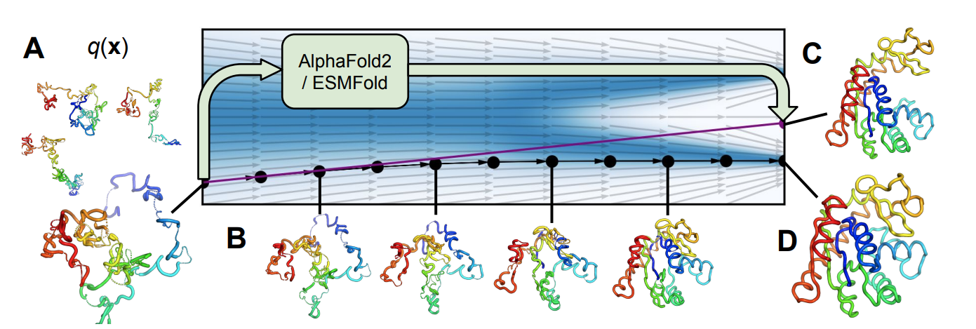
Recently, Jing et al, 2023 have also proposed using continuous flow matching for protein ensemble generation. Most of the components are similar to their previous work with diffusion models. They start from the harmonic prior and try to gradually refine the struture given the sequence. The main difference is that they use flow matching to generate the ensemble, which is more efficient and stable than diffusion models. Additionally, they slightly modify the vector field loss function to make it “FAPE”-like as in AlphaFold2.

Fig 5 from Jing et al, 2023: Illustration of the AlphaFlow/ESMFlow model. The model learns a vector field that generates a probability density path connecting the initial and final configurations in SE(3). The vector field model acitecture is adapted from AlphaFold/ESMFold.

Protein-ligand Binding

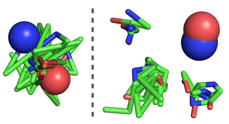
Stark et al, 2023 recently proposed HarmonicFlow, a novel method for protein-ligand binding, where they use flow matching to generate protein-ligand binding poses.

This method define the flow as a harmonic flow, which interpolate data distribution with a harmonic prior $p_0\left(\boldsymbol{x}_0\right) \propto \exp \left(-\frac{1}{2} \boldsymbol{x}_0^T \boldsymbol{L} \boldsymbol{x}_0\right)$ ($\boldsymbol{L}$ is the molecule graph Laplacian). It’s said that such prior can effectively introduce inductive bias on generated ligand strutcures. The flow is defined in coordinate space, and SE(3)-equivariant refinement Tensor Field Network (TFN) layers are used for vector field prediction.

Fig 6 from Stark et al, 2023: Comparison of the isotropic Gaussian (left) and the harmonic prior (right) in the multi-ligand binding task. Harmonic prior can effectively introduce inductive bias on separating ligand structures.

Single-cell Dynamics

Tong et al, 2023 also apply the flow matching framework for single-cell dynamics modeling, where they use flow matching for single-cell trajectory prediction. In their setup, they try to interpolate its distribution at time $t$ given times data at times $[0, t − 1]$, $[t + 1, T ]$. They use a 2D network to predict the vector field, which is then used to solve the ODE.

Fig 7 An illustration of the cell growth process.